Methodology¶

In this page we give a brief overview of the modelling process used in dynsity. We refer the interested reader to Takeuchi & Lin (2002) for more thorough details.

Background¶

The gas in a protoplanetary disk will rotate at a slightly sub-Keplerian velocity due to the support from the radial pressure gradient. In addition, the mass of the disk will contribute to the gravitational potential and speed the rotation of the disk, such that the total rotation is given by,

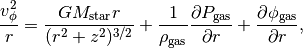
$\frac{v_{\phi}^2}{r} = \frac{GM_{\rm star}r}{(r^2 + z^2)^{3/2}} + \frac{1}{\rho_{\rm gas}} \frac{\partial P_{\rm gas}}{\partial r} + \frac{\partial \phi_{\rm gas}}{\partial r},$

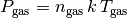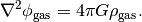
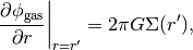
where, for an ideal gas, $P_{\rm gas} = n_{\rm gas} \, k \, T_{\rm gas}$ , and $\phi_{\rm gas}$ is the gravitational potential of the gas which satisfies

$\nabla^2 \phi_{\rm gas} = 4 \pi G \rho_{\rm gas}.$

If we are able to measure $v_{\phi}$ precisely, and are able to constrain both $z(r)$ and $T_{\rm gas}(r)$ observationally, we hope to

Place tight constraints on the dynamical mass of the star, $M_{\rm sun}$ .
Infer local changes in $P_{\rm gas}$ due to local deviations in $v_{\phi}$ , such as due to gaps in the gas surface density.
Constrain the dynamical mass of the disk after making some assumptions about how $\Sigma_{\rm gas}(r)$ varies.

The Model¶

Inputs¶

We assume that the user has been able to measure:

$v_{\phi}(r)$ - The deprojected rotational velocity of the gas as a function of radius in $[{\rm m\,s^{-1}}]$ .
$z(r)$ - The height of the emission surface as a function of radius in $[{\rm au}]$ .
$h_p(r)$ - The gas pressure scale height as a function of radius in $[{\rm au}]$ .
$T_{\rm gas}(r)$ - The gas temperature as a function of radius in $[{\rm K}]$ .

The emission surface can be derived either from fitting the rotation map, as in Keppler et al. (2019), or following the method in Pinte et al. (2018). The gas temperature is harder to measure, but optically thick lines like CO are useful as $T_{\rm B} = T_{\rm ex}$ . Optically thin lines may pose more of a challenge.

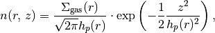
Gas Surface Density¶

We make the assumption that the gas surface density is well described by

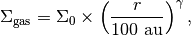
$\Sigma_{\rm gas} = \Sigma_0 \times \left( \frac{r}{100~{\rm au}}\right)^{\gamma},$

where we have neglected the often used exponential edge. The normalization of this term is given in terms of $M_{\rm disk}$ such that,

$\Sigma_0 = \frac{M_{\rm disk} \, r_0^{\gamma} \, (2 + \gamma)}{2 \pi \, (r_{\rm max}^2 - r_{\rm min}^2)},$

which means that $\gamma > -2$ . This means that for $\gamma \leq 2$ we have to calculate this numerically.

Note

With this approach, the inner radius of the fit is considered $r_{\rm min}$ and any disk mass inside this term will result in a slightly inflated $M_{\rm star}$ .

Gas Volume Density¶

To relate $\Sigma_{\rm gas}$ to $n({\rm H_2})$ we assume an isothermal vertical density profile,

$n(r,\, z) = \frac{\Sigma_{\rm gas}(r)}{\sqrt{2 \pi} h_p(r)} \cdot \exp\left(-\frac{1}{2}\frac{z^2}{h_p(r)^2} \right),$

where $h_p$ is the gas scale height. Unless there is some other observational constrain on $h_p$ , it is typically taken to be $h_p \, / \, r = 0.1$ . While this provides some degree of self-consistency between the models, significant changes in $z(r)$ can result in large deviation ins $n({\rm H_2})$ .

Note

There are different definitions of the $h_p$ which can vary by a factor of $\sqrt{2}$ . While this shouldn’t introduce a significant difference relative to the other uncertainties involved, it’s good to check.

Disk Self-Gravity¶

To calculate the self-gravity of the disk we can take the simplification of

$\left. \frac{\partial \phi_{\rm gas}}{\partial r} \right|_{r = r^{\prime}} = 2 \pi G \Sigma(r^{\prime}),$

which is appropriate when 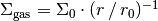$\Sigma_{\rm gas} = \Sigma_0 \cdot (r \, / \, r_0)^{-1}$ . However, testing showed that this was a poor approximation for anything where $\gamma \neq -1$ , even for small changes. Current approach is to solve numerically for this, but this is relatively slow (180 times slower…).

We can also consider the expansion:

$\phi_{\rm gas}(r) = -2 \pi G \int_{0}^{\infty} \int_{0}^{\infty} \Sigma(r^{\prime}) \, J_0(kr^{\prime}) \, r^{\prime} J_0(kr) \,{\rm d}r^{\prime} \,{\rm d}k$

where $J_0$ is the zeroth-order spherical Bessel function. This might not necessarily be quicker…

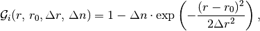
Perturbations in $n({\rm H_2})$ Profile¶

In dynsity we have two options for modelling $\delta n$ : either the product of multiple Gaussian perturbations,

$\delta n = \prod_{i}^N \mathcal{G}_i,$

where

$\mathcal{G}_i (r,\, r_0, \Delta r,\, \Delta n) = 1 - \Delta n \cdot \exp\left(-\frac{(r - r_0)^2}{2\Delta r^2}\right),$

or a $N^{\rm th}$ -order polynomial. Any number of perturbation terms can be added to the model for $n({\rm H_2})$ , however note that no perturbations will be added to the attached $T_{\rm gas}$ .

Warning

Currently we have no good way to bounding the coefficients for the polynomial perturbations so these should be ignored.